Support Vector Machines - SVM
Supervised Learning
Overview
What are Support Vector Machines (SVMs)?
-
A supervised learning algorithm that can solve complex classification and regression, plus detect outliers to determine boundaries between data points.
What are linear separators?
-
The concept of linear separators is a line otherwise known as the hyperplane being drawn between two different classes of points where both classes are contained on each side of the hyperplane.

Good Linear Separation
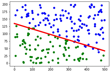
Bad Linear Separation
Kernel Functions
A kernel function takes in the data and transforms it into the form that SVM requires. The kernel acts as the window to manipulate data. The function takes the data from a non-linear decision surface to a linear equation in a high-dimension space.
There are different kinds of kernels:
-
Gaussian - Used to perform transformation if you have no prior knowledge about the data
-
Gaussian with Radial Basis Function (RBF) - Functions the same as a Gaussian kernel but adds radial basis to improve the transformation
-
Sigmoid - Two-layer perception model of a neural network, used as activation for artificial neurons
-
Polynomial - Represents similarity of vectors in a feature space over polynomial representation of the original variables
-
Linear - Used when data is linearly separable
Dot Products
The dot product is critical in the kernel because when you take the dot product of two vectors, which measures the similarity between the two vectors. By using dot products in the kernel, you can find points that are similar to each other and group them on the side of the hyperplane with the most similar neighbors.
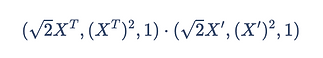
Polynomial Kernel

In this calculation, x and x' refer to two different observations in the data set. c determines the coefficient of the polynomial and d refers to the degree of the polynomial.
For example: Let's say we have a point (2, 4) with a coefficient of c = 1 and degree d = 2.
We would then write out the calculation to be and can be reduced into the following formula
Now, we can change this polynomial into a dot product of two vectors!
Now lets plug in our original point (2, 4). After simplifying the dot product down, the point would be mapped to (16, 64).
RBF Kernel

In this calculation, the nearest neighbors to the new point that needs to be classified are used.
In the formula, x and x' refer to two different observations. They are subtracted from each other and then squared to find their distance. The gamma is the scale of the influence the point has on the other and is multiplied by the squared distance.
Information sourced from: PennState, Microsoft & GeeksForGeeks
Data Prep
Supervised learning models always require labeled data. The data set must be split into a training and testing set. One that will train the model and one that will test the accuracy of the model.
One feature that SVM requires is having two mutually exclusive sets for the training and test set. For example, this algorithm would not run properly if the same data point existed in both the training and test set it is not a new data point for the algorithm and therefore the performance or accuracy of the model cannot be identified due to the lack of unfamiliarity of the data. Ideally, the test set should be of a similar distribution to the original training set but never seen before by the data set.
Another feature of data that SVM requires is numeric data. Due to the complexity of the formulas and math being performed, it cannot do that on anything but numbers.
Below are the training and test data sets that were made for the SVM algorithm. It is broken down as 70% training and 30% testing.

Training Data

Testing Data
Code & Results
The code will be completed and explored in Python.
RBF Kernel Exploration


Overall, pretty pleased with these results. 87.5% accuracy for the best case with 99 true positive identifications and 4 incorrect identifications.
As C increases to 100, the number of false negatives decreases pretty significantly, but as soon as C goes back up to 1000, the number goes back to the same as C=1.
The other thing of note is the amount of false positives being identified. As C increases the number of false positives triples!
Polynomial Kernel Exploration

Overall, not bad! The polynomial kernel was set with a coefficient of 1 and a degree of 2.
Polynomial with C=1 did the best so far at 88.33% with 99 true positive accuracy and 7 incorrect identifications.
The more C increased the worse the identifications got. True positive identifications took a significant hit as the value increased. False positives also took a big spike as C increased. The completely incorrect identifications stayed relatively constant which is interesting.


Sigmoid Kernel Exploration


As a result, the sigmoid kernel was the most consistent. As C increased, the accuracy didn't drop nearly as quickly as the kernels above.
The one thing that is interesting is that as C did increase, the amount of truly wrong identifications slowly went down, but the amount of false negative went up.
Conclusion
Overall, it was interesting to see just how well these algorithms performed at predicting whether or not a person would suffer from vertigo based on the other symptoms present. It seems that there are some consistencies in symptoms to predict migraine attacks but this is just a small dataset, it's nowhere near enough data to confirm that this truly can predict or not predict migraine symptoms.
Upon some further research, there was a study done on migraine sufferers and vertigo. It turns out that individuals who experience vertigo showed a higher lifetime prevalence of migraines than the control group. The symptom of vertigo still remains poorly defined but clearly, there is an association between intensity and vertigo based on findings in this SVM research.