Clustering
Unsupervised Learning
Overview
What is Clustering?
-
A technique that groups rows in a data set based on similar traits.
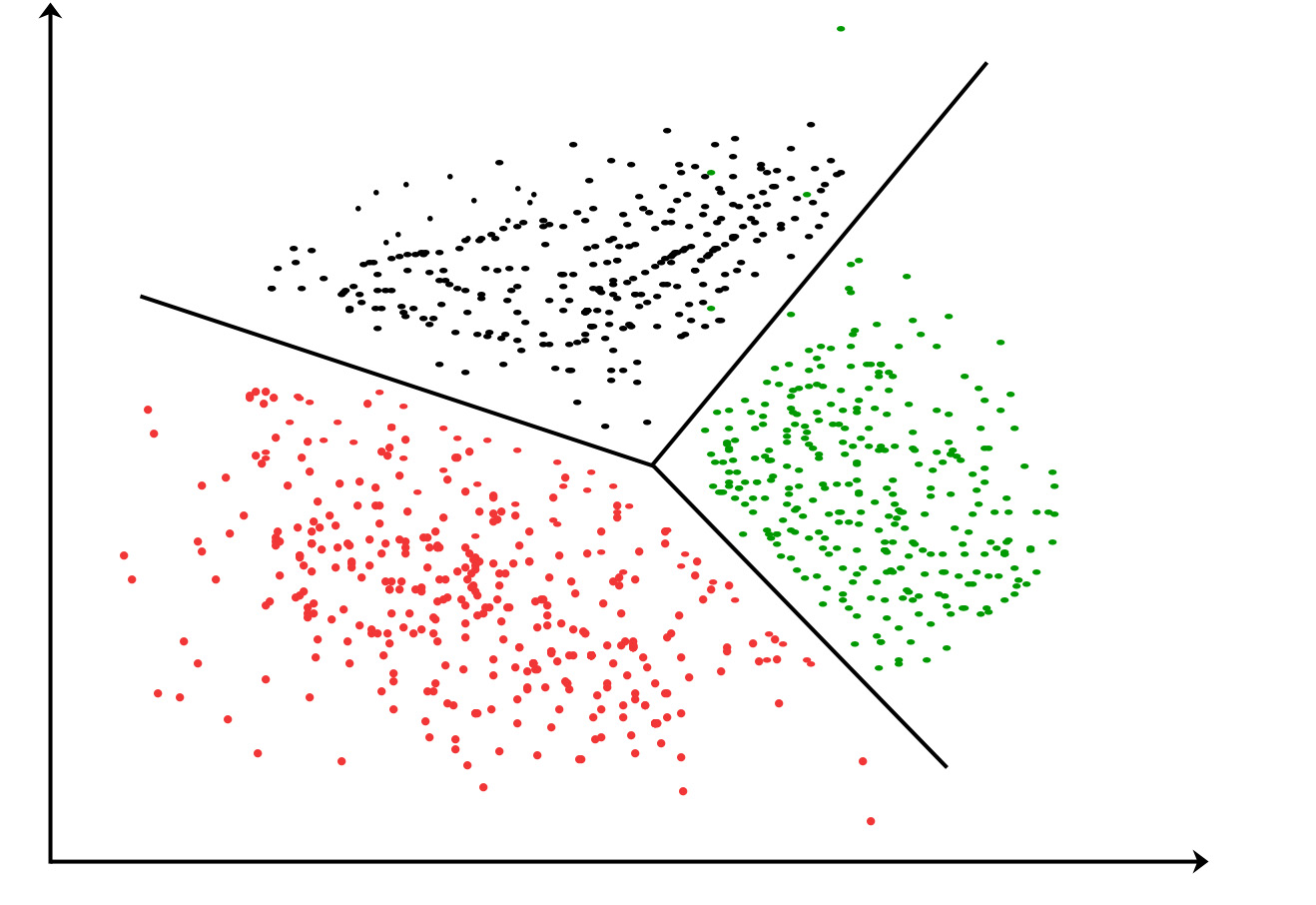
Partitional Clustering
Classifying observations of a data set into multiple groups based on similarities. Must specify the number of clusters (K) to generate.
Clustering methods:
-
K-means
-
K-medoids (PAM)
-
Clustering Large Applications Algorithm (CLARA)
Unique to Partitional Clustering:
-
Advanced knowledge of K by knowing the number of clusters desired.
-
The mean or median can represent the cluster center
-
Results produced will vary between iterations.
-
Less computationally expensive and works great for very large data sets.
Information sourced from: Global Tech Council & Medium
Hierarchical Clustering
Organizing observations into clusters based on similarities or distances.
Two types of hierarchical clustering:
-
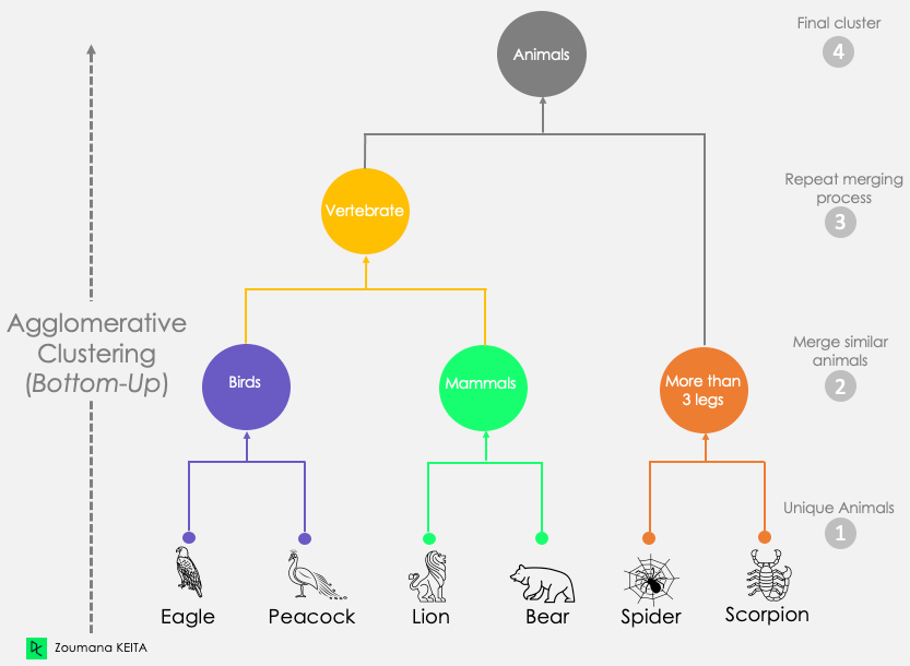
Agglomerative Clustering
-
Each data point is a separate cluster and then combines with all nearby clusters until one cluster is left.
-
-
Divisive clustering
-
Each data point is in one large cluster and the cluster divides until all data point is its own cluster.
-
Unique to Hierarchical Clustering:
-
Can choose any number of clusters.
-
Reproducible results
-
Set of nested clusters arranged as a tree
-
Doesn't work as well when clusters are hyper spherical
Information sourced from: Medium & Global Tech Council
Clustering methods being explored:
K-Means: Exploring the relationship between BMI and Age. If there is a relationship, what does each cluster show? Does having a higher BMI affect age at presentation? Is this a large factor in migraine onset?
Hierarchical Clustering: Exploring the relationship between migraine duration in days and frequency of migraines. Is there a trend in increased frequency and increased duration? Does having migraines more frequently signify less severe migraines or more severe migraines? Is duration the primary factor in migraine severity?
Data Prep
For clustering algorithms to run properly, only unlabeled numeric data. For the KMeans algorithm, the data set that will be used is the Harvard data set. This data set has been cleaned according to best practices, please refer back to the EDA tab for those procedures.
For additional cleaning on this algorithm, only columns Age at presentation and BMI were pulled and converted to numeric, plus the 2 NA values were supplemented with the means of each column. Below is a scatter visualization of the initial BMI vs Age along with a sample of the dataset.


Code
For K-Means clustering algorithms to run properly a K-value must be provided.
To determine the appropriate number of clusters needed, two methods can be tried. The Elbow Method and the Silhouette Method.

Optimal Clusters: k=4
For the elbow method, find the "elbow" of the curve in the graph.
The point on the graph at the elbow is the optimal number of clusters. In this case, the optimal number of clusters is 4.
Elbow Method
Silhouette Scores
For the silhouette method, the score evaluates the quality of the clustering results.
Silhouette scores range between [-1, 1] and follow the calculation.

The ideal silhouette score would be close to +1. This means that the boundaries of the clusters are far apart and are separated well. The opposite side -1 would mean the clusters are close together and hard to distinguish boundaries which could misclassify data. Just like the elbow test, k=4 was the optimal number of clusters.

Optimal Clusters: k=4
Next Best Clusters: k=6
Results
K-Means
k = 4, optimal

k = 6, next best

k = 3, sub-optimal

From the silhouette and elbow score, both determined the optimal k cluster values as 4. However, the silhouette score of 6 was pretty darn close too. Because of that fact, the k-means were run for both cluster values. The differences between the two are the clusters from BMI being below 30 being broken into two clusters and the outlier of BMI being almost 80 being a single element cluster. Visually, k=4 seems to be a good estimator for this data set, it has good boundaries for each cluster and breaks them up into distinguishing seconds. K-means additionally was run for k=3, which was sub-optimal, but the results produced weren't terrible! However, the upper chunk of cluster 1 in orange is pretty far away from the centroid, so definitely k = 4 accounting for that large gap makes more sense.
Hierarchical Clustering

Similarly, using hierarchical clustering with cosine similarity to measure the distance between points the dendrogram to the left shows that 4 distinct clusters can be formed against the Age and BMI of patients.
�
Interestingly, the right half of the dendrogram merges into one branch pretty quickly from the red into the blue line, almost implying that k=3 could be a valid cluster grouping as well.
Here is a visual heatmap representation of the data frame being used for the hierarchical clustering.
Based on the colors, the BMI is pretty substantially high across all ages!

Conclusion
From the two different clustering techniques and the resulting visualizations, there seems to be a trend between age and BMI. It seems that those who have a high BMI that is higher than 50, were diagnosed with chronic migraine at a much younger age than those who fell below a BMI of 30. Those who have a BMI between 40 and 50 were diagnosed initially in their late 20's to 60's. Those who have a BMI below 30 fluctuated heavily on when their initial diagnosis was.
Upon further personal research, according to a 2022 study on Headaches & Obesity, from 3,733 women the overall odds of migraines with a BMI classified as obese 30.0 or higher have a 1.5 times increased chance of suffering from migraines than those of a normal BMI.
Even though the sample size of the dataset was small, it followed similar conclusions from the study mentioned above. The study didn't mention age explicitly however mentioned that from adolescents aged 13-18, found that those who suffer migraines were 60% more likely to be overweight.